DES SN 5YR Tutorial Part 5: Lambda Dependent corrections
 Dark Energy Survey Supernova Program
Tutorial Part 5 Lambda Dependent corrections Contact author: Jason Lee
Here, we demonstrate how we obtain our magnitude corrections for the SHAPE (DCR + \(\lambda\)-dependent seeing) and COORD (DCR only) effects starting from the flux ratio tables and the altitude offset vs. g-i magnitude for each exposure.
[1]:
import warnings
warnings.filterwarnings("ignore")
[2]:
import numpy as np
import pandas as pd
import matplotlib.pyplot as plt
import astropy.units as u

from scipy.interpolate import RegularGridInterpolator
from astropy.coordinates import Angle, SkyCoord, AltAz, EarthLocation
from astropy.time import Time
from astropy.coordinates import Angle
from astropy.coordinates import AltAz, ICRS
from scipy.interpolate import interp1d
[3]:
earth_location = EarthLocation.of_site('ctio')
[4]:
DES_5YR_DCR_path = '../../../../DES-SN5YR/6_DCR_CORRECTIONS/'
1. SHAPE effect
(starting from the flux ratio (correct vs. uncorrected) tables)
Reading tables for SHAPE effect
flux ratio values table gives the flux ratio to when using the average color star as the PSF table columns = g-i values, AM_values, PSF FWHM values in arcseconds
[5]:
flux_ratio_values_g_table = np.load(DES_5YR_DCR_path + 'flux_ratio_values_g_table_DCR_shape.npy')
g_table_columns = np.load(DES_5YR_DCR_path + 'g_table_DCR_shape_xyz_columns.npy', allow_pickle=True)

flux_ratio_values_r_table = np.load(DES_5YR_DCR_path + 'flux_ratio_values_r_table_DCR_shape.npy')
r_table_columns = np.load(DES_5YR_DCR_path + 'r_table_DCR_shape_xyz_columns.npy', allow_pickle=True)
Using the GridInterpolator to 3D interpolate between the column values and flux ratio
[6]:
g_i_values_g, AM_values_g, psf_fwhms_g = g_table_columns
g_i_values_r, AM_values_r, psf_fwhms_r = r_table_columns
flux_interp_g_all = RegularGridInterpolator((g_i_values_g, AM_values_g, psf_fwhms_g), flux_ratio_values_g_table, bounds_error=False, fill_value = None)
flux_interp_r_all = RegularGridInterpolator((g_i_values_r, AM_values_r, psf_fwhms_r), flux_ratio_values_r_table, bounds_error=False, fill_value = None)
MCOR_220929 contains all the MAGCORs (both COORD and SHAPE) to be added to the uncorrected (SALT2 or SALT3) magnitudes
[7]:
MCOR_220929 = pd.read_csv(DES_5YR_DCR_path + 'DCRADJ_MAGCOR_v220929.csv')
MCOR_220929.head()
[7]:
| Unnamed: 0 | Unnamed: 0.1 | CID | EXPNUM | CCDNUM | MJD | BAND | TREST | LAMREST | SNR | ... | HA | dRA | dDEC | CUTS | ddRA | ddDEC | ADJOFF | PSF_FWHM_ASEC | MAGCOR_COORD | MAGCOR_SHAPE | |
|---|---|---|---|---|---|---|---|---|---|---|---|---|---|---|---|---|---|---|---|---|---|
| 0 | 0 | 3627 | 1246281 | 255449 | 51 | 56614.0731 | g | 49.2 | 3613.5 | 1.7 | ... | b'-02:46:38.520' | 0.017590 | 0.004682 | True | 0.038003 | 0.009945 | 0.039283 | 0.927 | -0.002618 | 0.002402 |
| 1 | 1 | 3655 | 1246281 | 255888 | 51 | 56615.0961 | g | 49.9 | 3613.5 | 1.8 | ... | b'-02:09:31.400' | 0.012814 | 0.003172 | True | 0.033227 | 0.008435 | 0.034281 | 0.997 | -0.001724 | 0.001877 |
| 2 | 2 | 4066 | 1246281 | 238052 | 51 | 56559.1905 | g | 8.1 | 3613.5 | 5.0 | ... | b'-03:33:58.020' | -0.022856 | -0.007003 | True | -0.002442 | -0.001740 | 0.002999 | 1.330 | -0.000007 | -0.004349 |
| 3 | 3 | 4080 | 1246281 | 238984 | 51 | 56563.2002 | g | 11.1 | 3613.5 | 9.0 | ... | b'-03:04:13.260' | -0.017628 | -0.004924 | True | 0.002786 | 0.000338 | 0.002806 | 1.344 | -0.000006 | -0.003640 |
| 4 | 4 | 4108 | 1246281 | 242477 | 51 | 56575.1914 | g | 20.1 | 3613.5 | 5.2 | ... | b'-02:29:35.140' | 0.001841 | 0.000471 | True | 0.022254 | 0.005734 | 0.022981 | 0.925 | -0.000900 | 0.001309 |
5 rows × 26 columns
SHAPE example for one candidate at a particular exposure
[8]:
ind = 0

EX_g_i = MCOR_220929.iloc[ind]['MAG_MODEL_g'] - MCOR_220929.iloc[ind]['MAG_MODEL_i']
EX_AM = MCOR_220929.iloc[ind]['AIRMASS']
EX_PSF_FWHM = MCOR_220929.iloc[ind]['PSF_FWHM_ASEC']
[9]:
# Convert flux ratio to magnitude correction

EX_MAG_COR_SHAPE = -2.5/np.log(10) * (1. - flux_interp_g_all([EX_g_i, EX_AM, EX_PSF_FWHM]))
[10]:
# Compare with MAGCOR file

print(EX_MAG_COR_SHAPE, MCOR_220929.iloc[ind]['MAGCOR_SHAPE'])
[0.00240155] 0.0024015458236172
2. COORD effect
(starting from altitude shift vs. g-i magnitude)
We first start from reading tables for COORD
[11]:
coord_dictionary = pd.read_csv(DES_5YR_DCR_path + 'DCR_dictionary.csv')
mag_corr_vs_offset = np.loadtxt(DES_5YR_DCR_path + 'mmag_vs_fracpsf_Moffat3.txt')
[12]:
DCR_coord_table = pd.read_csv(DES_5YR_DCR_path + 'DCR_coord_table.csv')
[13]:
DES_bands = ['g', 'r', 'i', 'z']
[14]:
where_band = []
for i in range(len(DES_bands)):
    where_band.append(np.where(MCOR_220929['BAND'] == DES_bands[i][0]))
COORD example
[15]:
expnums = MCOR_220929['EXPNUM'].values

g_i_vals = MCOR_220929['MAG_MODEL_g'].values - MCOR_220929['MAG_MODEL_i'].values
Altitude slope and y intercept values for each exposure
[16]:
slope_y_int_vals = np.zeros([2, len(MCOR_220929)])

for i in range(len(slope_y_int_vals[0])):
    dict_ = coord_dictionary[coord_dictionary['EXPNUM'] == expnums[i]]
    slope_y_int_vals[0][i] = dict_['SLOPE_ALT']
    slope_y_int_vals[1][i] = dict_['YINT_ALT']
Convert to altitude shifts: see Figure 5 of Lee & Acevedo et. al (2023) https://arxiv.org/abs/2304.01858
[17]:
alt_shift_vals = g_i_vals * slope_y_int_vals[0] + slope_y_int_vals[1]
[18]:
def sky_to_alt_az_coords(SN_fid_pos, mjd, loc = earth_location):
    coord0 = SkyCoord(SN_fid_pos[0] * u.deg, SN_fid_pos[1] * u.deg)
    aa = AltAz(location=loc, obstime=Time(mjd, scale = 'utc', format = 'mjd', location = loc))
    alt, az = coord0.transform_to(aa).alt, coord0.transform_to(aa).az
    return alt, az
[19]:
def alt_az_to_sky_coords(alt, az, mjd, loc=earth_location):
    # Create AltAz object
    aa = AltAz(alt=alt*u.deg, az=az*u.deg, location=loc, obstime=Time(mjd, format='mjd'))

    # Transform AltAz to Equatorial coordinates (ICRS)
    equatorial_coords = aa.transform_to(ICRS())

    # Extract RA and DEC
    ra, dec = equatorial_coords.ra, equatorial_coords.dec

    return ra, dec
[20]:
nominal_RA_vals, nominal_DEC_vals = MCOR_220929['RADEG'].values, MCOR_220929['DECDEG'].values
mjds = MCOR_220929['MJD'].values

alt_deg, az_deg = sky_to_alt_az_coords([nominal_RA_vals, nominal_DEC_vals], mjds)
[21]:
lat = earth_location.lat.value

sinq = -np.cos(lat*u.deg)*np.sin(az_deg)/np.cos(nominal_DEC_vals*u.deg)
cosq = (np.sin(lat*u.deg)-np.sin(nominal_DEC_vals*u.deg)*np.sin(alt_deg))/(np.cos(nominal_DEC_vals*u.deg)*np.cos(alt_deg))
[22]:
# Convert altitude shifts to dRA, dDEC

dRA, dDEC = alt_shift_vals*sinq, alt_shift_vals*cosq
[23]:
# Checking dRA dDEC with csv file

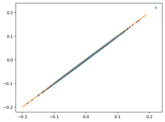
plt.plot(dRA[np.where(MCOR_220929['BAND'] == 'g')[0]], MCOR_220929[MCOR_220929['BAND'] == 'g']['dRA'], '.')

plt.plot(np.arange(-0.2, 0.2, 0.01), np.arange(-0.2, 0.2, 0.01))
[23]:
[<matplotlib.lines.Line2D at 0x16a0e82c0>]
[24]:
MCOR_220929['CID'].unique()
[24]:
array([1246281, 1246430, 1246527, ..., 1959025, 1960031, 1974019])
[25]:
cid, band = 1246281, 'g'
where_cid_band = np.where((MCOR_220929['CID'] == cid) & (MCOR_220929['BAND'] == band))[0]
SNR_where_cid_band = MCOR_220929['SNR'][where_cid_band]
[26]:
# COORD shift in RA, DEC with respect to the SNR^2 weighted average

ddRA_cid_band, ddDEC_cid_band = dRA[where_cid_band] - np.average(dRA[where_cid_band], weights = SNR_where_cid_band**2), dDEC[where_cid_band] - np.average(dDEC[where_cid_band], weights = SNR_where_cid_band**2)
[27]:
# Check ddRA, ddDEC with csv file

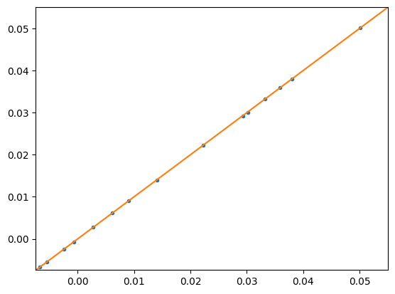
plt.plot(ddRA_cid_band, MCOR_220929['ddRA'][where_cid_band], '.')
plt.plot(np.arange(-0.2, 0.2, 0.01), np.arange(-0.2, 0.2, 0.01))
plt.xlim(ddRA_cid_band.min()*1.1, ddRA_cid_band.max()*1.1)
plt.ylim(MCOR_220929['ddRA'][where_cid_band].min()*1.1, MCOR_220929['ddRA'][where_cid_band].max()*1.1)
[27]:
(-0.00738635890821312, 0.0551164154097413)
[28]:
# Total OFFSET

ADJOFF_cid_band = np.sqrt(ddRA_cid_band**2 + ddDEC_cid_band**2)
print(ADJOFF_cid_band, MCOR_220929['ADJOFF'][where_cid_band].values)
[0.03932834 0.03434253 0.00299094 0.00280766 0.02298685 0.03114068
 0.01049225 0.03709824 0.03020881 0.05214196 0.00630405 0.00941435
 0.01432433 0.00558399 0.00694969] [0.0392828  0.03428121 0.00299867 0.0028061  0.02298113 0.03108189
 0.01050769 0.03708267 0.03018175 0.05217067 0.00628068 0.00938201
 0.01433384 0.00562435 0.00692192]
[29]:
# Convert to offset in multiples of PSF FWHM (Figure 4 of Lee & Acevedo et al. (2023))

OFF_PSF_FWHM_cid_band = ADJOFF_cid_band/MCOR_220929['PSF_FWHM_ASEC'][where_cid_band].values
[30]:
# Interpolate mag correction by offset

coord_off, magoff = mag_corr_vs_offset[0], mag_corr_vs_offset[1]
magoff_interp = interp1d(coord_off, magoff)
[31]:
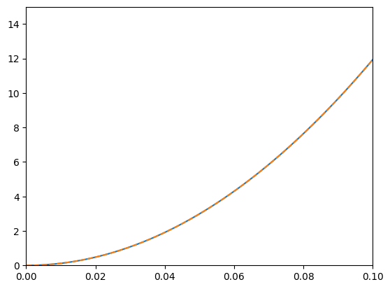
# Figure 4 for the Moffat profile

plt.plot(mag_corr_vs_offset[0], mag_corr_vs_offset[1])
plt.plot(coord_off, magoff_interp(coord_off), ls = '--')
plt.xlim(0, 0.10)
plt.ylim(0, 15)
[31]:
(0.0, 15.0)
[32]:
# Compare with csv file

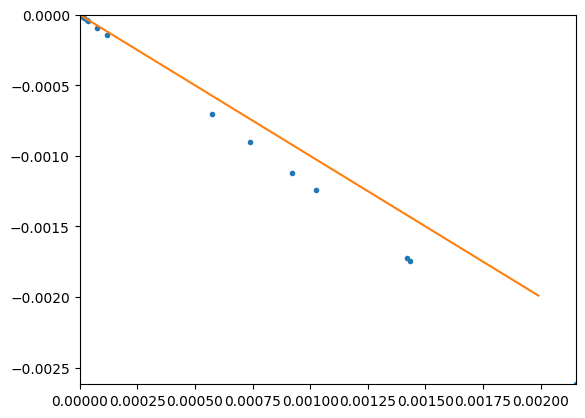
plt.plot(magoff_interp(OFF_PSF_FWHM_cid_band)*1e-3, MCOR_220929['MAGCOR_COORD'][where_cid_band].values, '.')
plt.plot(np.arange(0, 0.002, 0.00001), -np.arange(0, 0.002, 0.00001))

print(magoff_interp(OFF_PSF_FWHM_cid_band)*1e-3/MCOR_220929['MAGCOR_COORD'][where_cid_band].values)

plt.xlim(0, magoff_interp(OFF_PSF_FWHM_cid_band).max()*1e-3)
plt.ylim(MCOR_220929['MAGCOR_COORD'][where_cid_band].values.min(), 0)
[-0.82161476 -0.82300294 -0.91907314 -0.94210969 -0.82027624 -0.82292534
 -0.8261532  -0.82059541 -0.82148971 -0.81899311 -0.84834005 -0.83548809
 -0.822037   -0.83689179 -0.84754167]
[32]:
(-0.002618313475896, 0.0)