DES SN 5YR Tutorial Part 3: Load DES SN Classification
 Dark Energy Survey Supernova Program
Tutorial Part 3 Load SN classfication Contact author: Bruno Sánchez (bsanchez@cppm.in2p3.fr)
This tutorial is intended to show how to load the data from the classification files provided with this release.
We will load the package utils module and data module.
utils provides functionality to read the data formats
data provides with the location of the downloaded DR files.
[1]:
import warnings
warnings.filterwarnings("ignore")
[2]:
import os
import pandas as pd
import numpy as np
from matplotlib import pyplot as plt
[3]:
from dessndr import utils, data
This is the loacation of the cloned DR repository in our system:
[4]:
print(data.DES5YRDR_DATA)
/Users/sanchez/Data/DES/DESSNDR/DES-SN5YR
[5]:
probas = pd.read_csv(os.path.join(data.DES5YRDR_DATA, '3_CLASSIFICATION/DES_classification.csv'))
[6]:
probas
[6]:
| CID | CIDint | PROB_SCONE | PROB_SNIRFV19 | PROB_SNNDESCC | PROB_SNNJ17 | PROB_SNNV19 | |
|---|---|---|---|---|---|---|---|
| 0 | 1246275 | 1246275 | 0.9902 | 0.8486 | 1.0000 | 0.9999 | 1.0000 |
| 1 | 1246281 | 1246281 | 0.9432 | 1.0000 | 1.0000 | 0.9999 | 1.0000 |
| 2 | 1246314 | 1246314 | 0.9891 | 0.7823 | 0.9993 | 0.9970 | 0.9998 |
| 3 | 1246527 | 1246527 | 0.9757 | 1.0000 | 0.9997 | 0.9998 | 1.0000 |
| 4 | 1246529 | 1246529 | 0.9549 | 0.9407 | 0.9996 | 0.9993 | 1.0000 |
| ... | ... | ... | ... | ... | ... | ... | ... |
| 1630 | 1948484 | 1948484 | 0.8789 | 0.9146 | 0.9640 | 0.9935 | 0.9996 |
| 1631 | 1950024 | 1950024 | 0.9000 | 0.9380 | 0.9999 | 0.9937 | 0.9355 |
| 1632 | 1950043 | 1950043 | 0.9573 | 0.9454 | 0.9964 | 0.9874 | 0.2608 |
| 1633 | 1959025 | 1959025 | 0.9867 | 0.8921 | 0.9996 | 0.9996 | 0.9998 |
| 1634 | 1968046 | 1968046 | 1.0000 | 0.9225 | 1.0000 | 0.9998 | 1.0000 |
1635 rows × 7 columns
[7]:
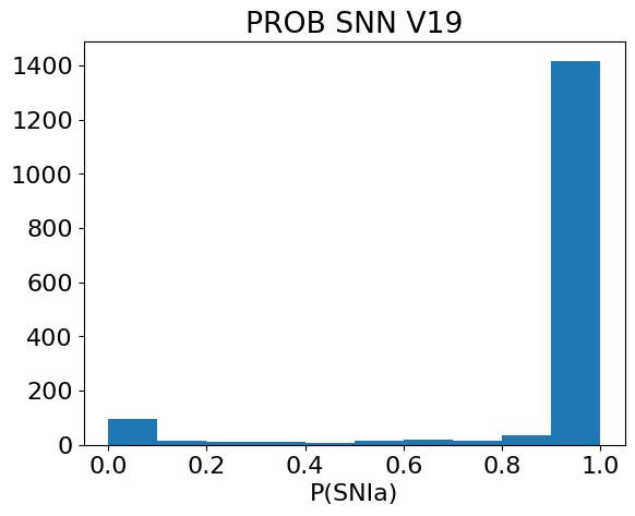
plt.hist(probas.PROB_SNNV19)
plt.title('PROB SNN V19')
plt.xlabel('P(SNIa)')
[7]:
Text(0.5, 0, 'P(SNIa)')
Now we are going to load the DES photometry files:
[8]:
phot_version = os.path.join(
    data.DES5YRDR_DATA_ROOT,
    'DES-SN5YR/0_DATA/DES-SN5YR_DESDR/DES-SN5YR_DESDR'
)
phot = utils.PhotFITS(phot_version)
Let’s select a few of the high probability!
[9]:
random_snias = probas[probas.PROB_SNIRFV19==1.].sample(3).CID.values
[10]:
from dessndr import plot
[11]:
lc = phot.get_lc(random_snias[0])
[12]:
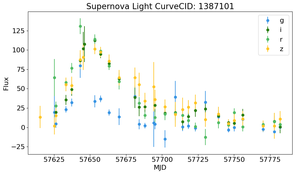
plot.plot_sn_light_curve(lc, CID=random_snias[0], figsize=(10, 6))
[12]:
(<Figure size 1000x600 with 1 Axes>,
 <Axes: title={'center': 'Supernova Light CurveCID: 1387101'}, xlabel='MJD', ylabel='Flux'>)
[13]:
lc = phot.get_lc(random_snias[1])
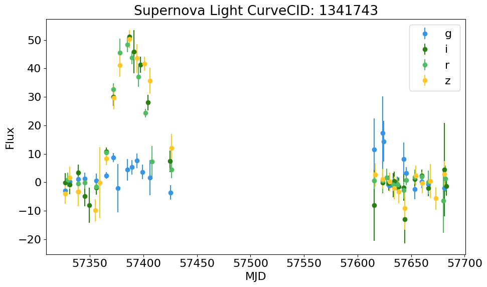
plot.plot_sn_light_curve(lc, CID=random_snias[1], figsize=(10, 6))
[13]:
(<Figure size 1000x600 with 1 Axes>,
 <Axes: title={'center': 'Supernova Light CurveCID: 1341743'}, xlabel='MJD', ylabel='Flux'>)
[14]:
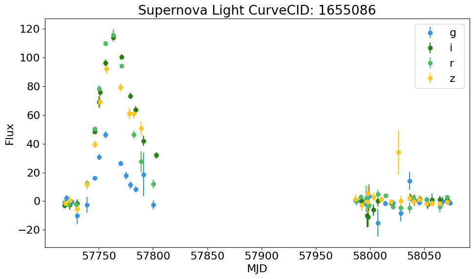
lc = phot.get_lc(random_snias[2])
plot.plot_sn_light_curve(lc, CID=random_snias[2], figsize=(10, 6))
[14]:
(<Figure size 1000x600 with 1 Axes>,
 <Axes: title={'center': 'Supernova Light CurveCID: 1655086'}, xlabel='MJD', ylabel='Flux'>)
Now let’s check a few of the bad ones!
[15]:
random_snias = probas[probas.PROB_SNIRFV19<0.1].sample(3).CID.values
[16]:
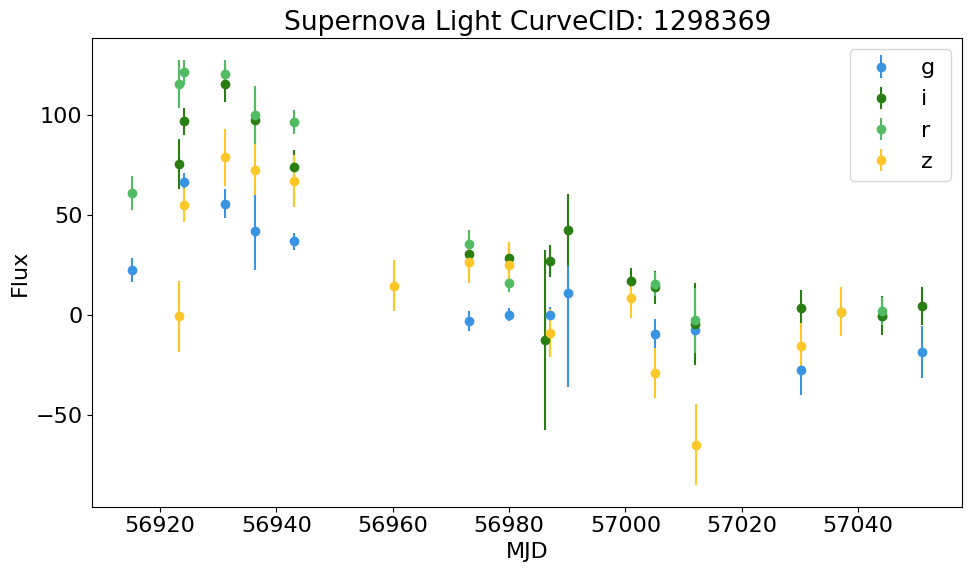
lc = phot.get_lc(random_snias[0])
plot.plot_sn_light_curve(lc, CID=random_snias[0], figsize=(10, 6))
[16]:
(<Figure size 1000x600 with 1 Axes>,
 <Axes: title={'center': 'Supernova Light CurveCID: 1298369'}, xlabel='MJD', ylabel='Flux'>)
[17]:
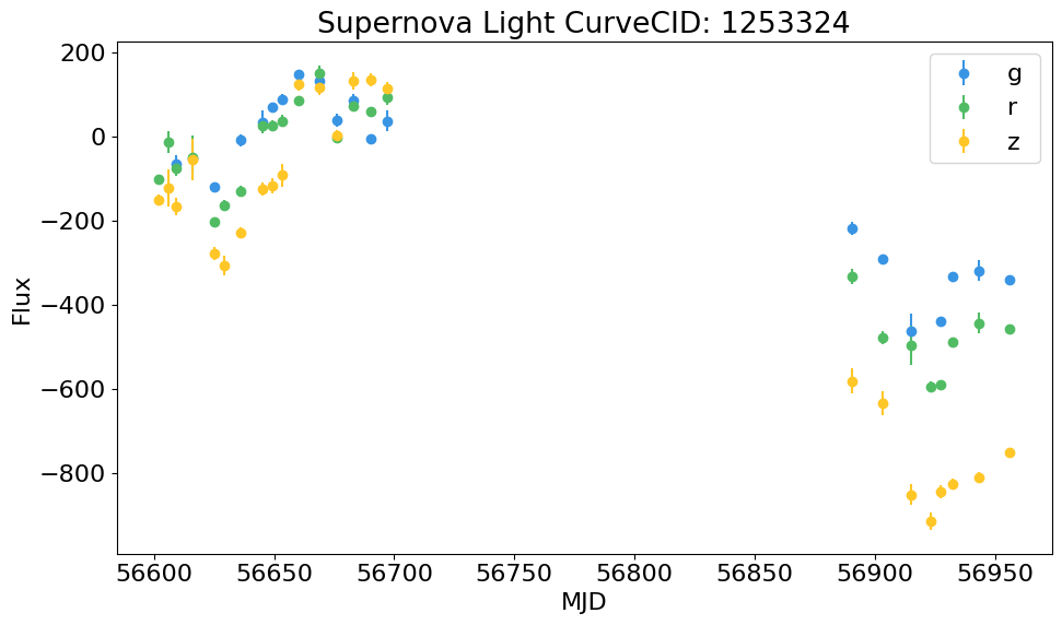
lc = phot.get_lc(random_snias[1])
plot.plot_sn_light_curve(lc, CID=random_snias[1], figsize=(10, 6))
[17]:
(<Figure size 1000x600 with 1 Axes>,
 <Axes: title={'center': 'Supernova Light CurveCID: 1253324'}, xlabel='MJD', ylabel='Flux'>)
[18]:
lc = phot.get_lc(random_snias[2])
plot.plot_sn_light_curve(lc, CID=random_snias[2], figsize=(10, 6))
[18]:
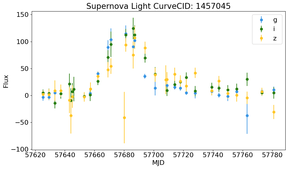
(<Figure size 1000x600 with 1 Axes>,
 <Axes: title={'center': 'Supernova Light CurveCID: 1457045'}, xlabel='MJD', ylabel='Flux'>)